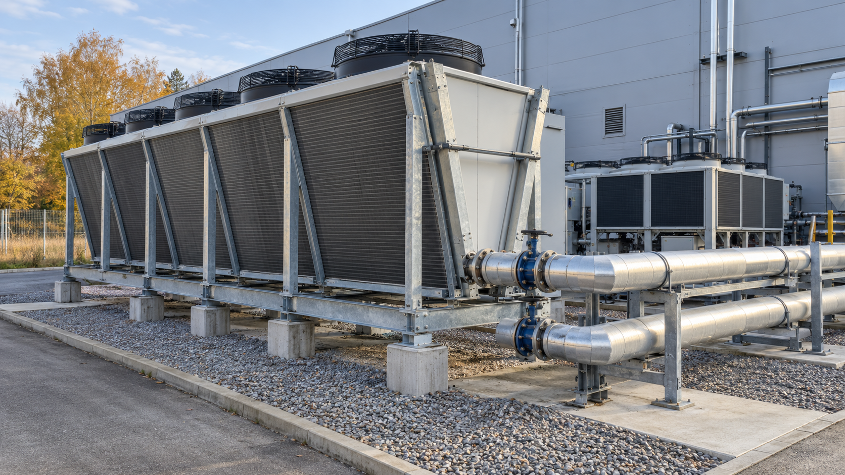
Free cooling uses a cooler environment to remove heat from an industrial process, reducing the need to run a chiller’s compressors. It does not mean cooling without electricity: pumps, fans and controls still operate. The actual benefit depends on the required fluid temperatures, the cooling demand profile and the efficiency of the entire system at different times of the year.
How does free cooling work in industry?
In a conventional chilled-water system, a chiller removes heat from the fluid through a compressor-based refrigeration cycle. With free cooling, cooler outdoor air removes heat through a dry cooler or a heat exchanger integrated into the chiller. Under sufficiently favourable conditions, the compressors can be switched off. Otherwise, free cooling may only pre-cool the fluid, leaving the chiller to supply the remaining cooling capacity.
Applications include cooling machines, production equipment, moulds, process loops and other loads that operate outside the summer months. This should not be confused with every form of using cool outdoor air for building ventilation. Here we focus on free cooling for chilled-water installations and industrial liquid circuits, rather than designing an entire refrigeration system. Our article on industrial refrigeration provides broader context on equipment and cooling loads.
When is the outdoor air cool enough?
Heat must flow from the warmer fluid to a cooler heat sink, but an outdoor air temperature below the return-fluid temperature does not, by itself, guarantee full free cooling. The temperature difference needed for heat transfer, heat exchanger capacity, flow rate, fouling and losses across subsequent components must also be considered.
For example, assume a process requires supply water at 14°C and returns it at 19°C. If, at the flows and load under consideration, the dry cooler needs an assumed 5 K difference between outdoor air and the leaving fluid temperature, an outdoor temperature of 6°C may allow sufficient margin for full cooling. At 12°C, this simplified example suggests the return water might be cooled to around 17°C, but not to the required 14°C. The chiller would then need to provide additional cooling. The 5 K figure is an assumption for this example, not a universal dry-cooler parameter; actual temperatures depend on the equipment performance curves.
| Operating mode | Technical requirement | What consumes electricity? |
|---|---|---|
| Full free cooling | The heat exchanger arrangement meets the required load at the specified supply temperature. | Primarily pumps, fans, controls and any auxiliary equipment; compressors remain off. |
| Partial free cooling | Ambient conditions allow the fluid to be pre-cooled but cannot meet the entire cooling demand. | Auxiliary drives and a chiller operating at reduced load. |
| Mechanical cooling | Free cooling provides no useful capacity under the prevailing conditions. | The chiller, pumps and other drives required to operate the installation. |
Daikin’s overview of free-cooling solutions also describes the progression from mechanical cooling through partial to full free cooling. Evaporative cooling needs to be assessed differently from dry coolers: wet-bulb temperature and water management also matter. Temperature thresholds should therefore not be transferred between different technologies.
Free-cooling availability must be calculated hour by hour
Knowing that a region experiences many hours of low outdoor temperatures is not enough to justify an investment. During those same hours, the plant must actually need cooling, and the equipment must be able to deliver the required capacity at the specified conditions. A plant operating three shifts throughout the year will usually have different potential from a facility that needs cooling only during summer production.
The analysis requires, at a minimum, the following data:
- Cooling load profile over time: cooling capacity or energy in successive hours, production changes and shutdowns.
- Supply and return temperatures and the permissible deviations required by the process.
- Fluid flow rate, pump characteristics, pressure losses and any differences between circuits.
- Weather data from as close to the equipment location as possible and corresponding to the plant’s operating hours.
- Heat exchanger and dry-cooler performance data for the relevant temperatures, flows and fan control settings.
- Electrical power demand of the chiller and auxiliary drives at the corresponding operating points.
Potential sources of external data include measurement and observation data from Poland’s IMGW-PIB and hourly ERA5 reanalysis data provided by Copernicus. Accurate equipment selection must allow for differences between weather-station or gridded data and the conditions at the dry cooler’s air intake, for example on a heat-absorbing factory roof.
How can cooling load be calculated from measurements?
For a water circuit, the approximate rate of heat removal can be calculated as follows: Q [kW] ≈ 1.163 × flow rate [m³/h] × temperature difference [K]. A flow rate of 17.2 m³/h and a temperature difference of 5 K give approximately 100 kW. This approximation applies to water at typical operating temperatures; glycol solutions require the appropriate specific heat capacity and density for their actual composition and temperature.
For each simulated hour, establish the process cooling load, the dry cooler’s available capacity under current conditions and the total electrical demand of each system option. Only the combined hourly results reveal the hours of full and partial free cooling, the amount of cooling supplied by it and the electricity needed to deliver that cooling.
Full and partial free cooling need appropriate controls
The controller should select the operating mode according to the achievable supply temperature, cooling demand and electrical power balance. A typical sequence involves starting the free-cooling circuit, adjusting flow rates and fan speeds, and then gradually increasing or reducing the chiller’s contribution as needed. Trane also describes how a dry cooler can work with an existing chilled-water installation.
In practice, check the following:
- switching hysteresis to prevent the chiller and valves from short-cycling as temperatures change slightly;
- temperature and flow sensors on both sides of the heat exchanger, including the reliability of their readings;
- minimum flow requirements through the chiller, heat exchanger and end-use equipment;
- maintaining process conditions as the first priority during start-up, shutdown and faults;
- freeze protection, hydraulic bypasses and the procedure for returning to mechanical cooling;
- logging operating modes, temperatures, flows, power and alarms in the monitoring system.
Not every situation with theoretical pre-cooling potential saves energy. If the additional pump and fan operation uses more electricity than the compressor saves, the controller should not force mixed-mode operation merely because the outdoor temperature has dropped.
Pumps, fans and glycol can change the energy balance
The word “free” refers to the cooling source, not to the cost of running the system. Adding a dry cooler may also mean additional fans, an outdoor-loop pump, another plate heat exchanger, valves and greater hydraulic resistance. Energy savings must be calculated for the entire system, including existing and added drives, rather than by simply comparing compressor power with fan power. The U.S. Department of Energy discusses water-side economizers that, depending on their arrangement, can replace chiller operation or pre-cool the water. Although the example concerns data-centre cooling, the principle of assessing the whole system applies to industrial processes as well.
A circuit exposed to freezing temperatures needs protection appropriate to local conditions and the manufacturer’s documentation. A water-glycol mixture is often used. Because this changes the thermal and hydraulic properties of the fluid, pump capacity and pressure losses must not be assumed to be the same as with pure water. One option is to create a separate outdoor glycol loop, isolated from the process circuit by a heat exchanger. This limits glycol in the process circuit but adds thermal resistance and may require another pump. Daikin’s solution documentation illustrates glycol-based options and an outdoor circuit separated from the customer’s system.
How much electricity could be saved? An example for one operating period
Assume an industrial circuit needs 100 kW of cooling for 1000 selected hours when conditions permit full free cooling. For a fair comparison, the cooling delivered and required temperatures are identical in both cases. The electrical power figures below are illustrative assumptions covering all significant drives in each configuration; they are not measured results from a particular plant.
| Parameter | Chiller only | Full free cooling |
|---|---|---|
| Cooling capacity delivered | 100 kW | 100 kW |
| Total electrical power: compressors, pumps, fans and other drives | 35 kW | 13 kW |
| Operating time in the hours analysed | 1000 h | 1000 h |
| Electrical energy | 35 000 kWh | 13 000 kWh |
The difference is (35 − 13) kW × 1000 h = 22 000 kWh, or 22 MWh of electricity in those hours. This is not automatically the plant’s annual saving. During the remaining hours, the system may operate in partial free-cooling mode or use only mechanical cooling, with power consumption depending on the actual load and controls.
The financial assessment must then include investment, operation and maintenance costs, possible glycol replacement and the value of electricity during the hours when demand actually falls. Compare options for a warmer year and lower production load as well. If the investment is to be justified through energy savings, an energy efficiency audit with a clearly defined method for comparing the baseline and retrofit options may be appropriate.
Which plants are suitable for a retrofit, and where is caution needed?
The most promising installations have year-round or extended cooling seasons, a steady cooling load and supply temperatures high enough for ambient conditions to meet them during many hours. Circuits removing heat from production equipment, for example, may offer favourable conditions. Each process must nevertheless be assessed individually: raising the water temperature too much may adversely affect product quality or machinery operating conditions.
More caution is needed where cooling is required almost exclusively on hot days, the process needs very low supply temperatures, there is no space for a dry cooler, or connecting a new heat exchanger would significantly increase pressure losses and retrofit complexity. It is also worth checking whether waste heat can be put to productive use: in some cases, industrial heat recovery deserves a separate comparison with rejecting that heat to the environment. These are different energy decisions and may compete during certain hours.
What should be checked before investing and during commissioning?
- Define the system boundary. Specify which chillers, circuits, pumps and end uses are included in the comparison so auxiliary consumption is not overlooked.
- Collect measurements from representative operating periods. Record flows, temperatures, electrical power, process load and information about production changes and shutdowns.
- Develop an hourly energy balance. Match the operating hours of cooling loads with weather and equipment performance data to determine the shares of full, partial and mechanical cooling.
- Check technical constraints. Verify freeze protection, pump and heat exchanger pressure losses, installation space, noise, service access and the ability to maintain process conditions during faults.
- Define acceptance criteria. Under suitable operating conditions, verify supply temperature, flow rate, control mode and the electrical power of the whole installation. Ensure data are logged so performance can be assessed after the retrofit.
From an auditor’s perspective, the key is to distinguish two questions: how much cooling can be delivered without compressors, and how much electricity will the installation actually stop consuming? Thermal sizing answers the first; only a system-wide balance based on plant operating data answers the second.
How should you begin assessing free cooling at your plant?
Start with a straightforward description of the installation: what is cooled, during which hours, the required supply and return temperatures, and which equipment and measurements are already available. This helps establish whether the priority is load-profile analysis, a controls review or a comparison of retrofit options. You do not need every measurement before the first conversation. If you would like to organise the data and define the scope of such an assessment, contact Energy Trend.
Technical sources and data for the analysis
- Daikin — free-cooling solutions for air-cooled chillers: circuit configurations and transitions between operating modes.
- Trane — free cooling: the operating principle of a dry cooler connected to a chilled-water installation.
- U.S. Department of Energy — Cooling Water Efficiency Opportunities: water-side economizers installed in parallel or in series with a chiller.
- IMGW-PIB — public data: information on access to meteorological observations and archives.
- Copernicus Climate Data Store — ERA5: hourly weather reanalysis data, subject to spatial-resolution limitations.